Introduction to independence and conditional probability

February 21, 2020

⊕
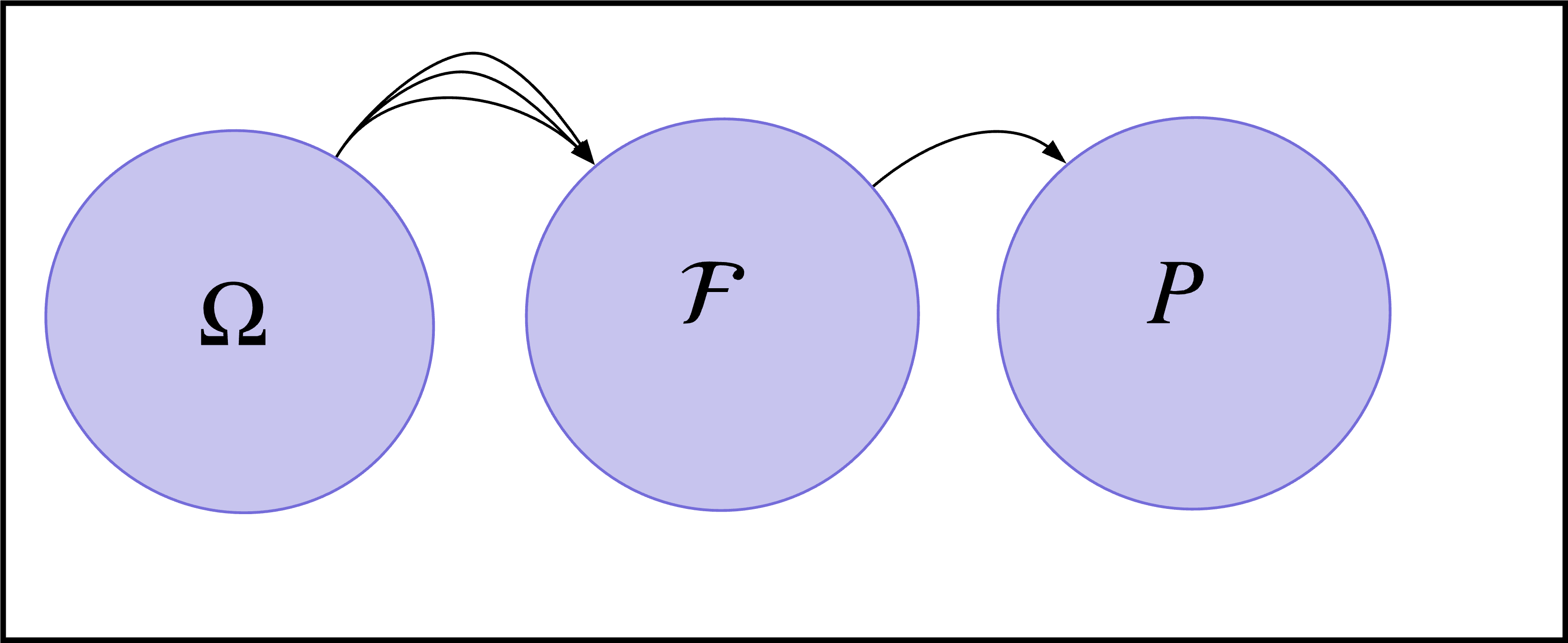
Figure 1: Here, the elements of a sample space get mapped onto an event space (ie. a collection of subsets from the sample space). These event elements get uniquely mapped onto a probability space.

Let’s expand our intuition for probability. To do so, we have to extend our understanding of sets as well. Recall from the previous entry on Probability Spaces that the glue that held the intuition and mathematical explanations was the concept of sets.

Currently, we know that probabilities under a Probability Triplet $(\Omega, \mathcal{F}, P)$ maps elements of an event space $\mathcal{F}$ to probabilities P, which are real numbers in $\mathbb{R}$. In order to ease the notation to be more readable, let’s say the probability of events $A \in \mathcal{F_A}$ to be $P(A)$.

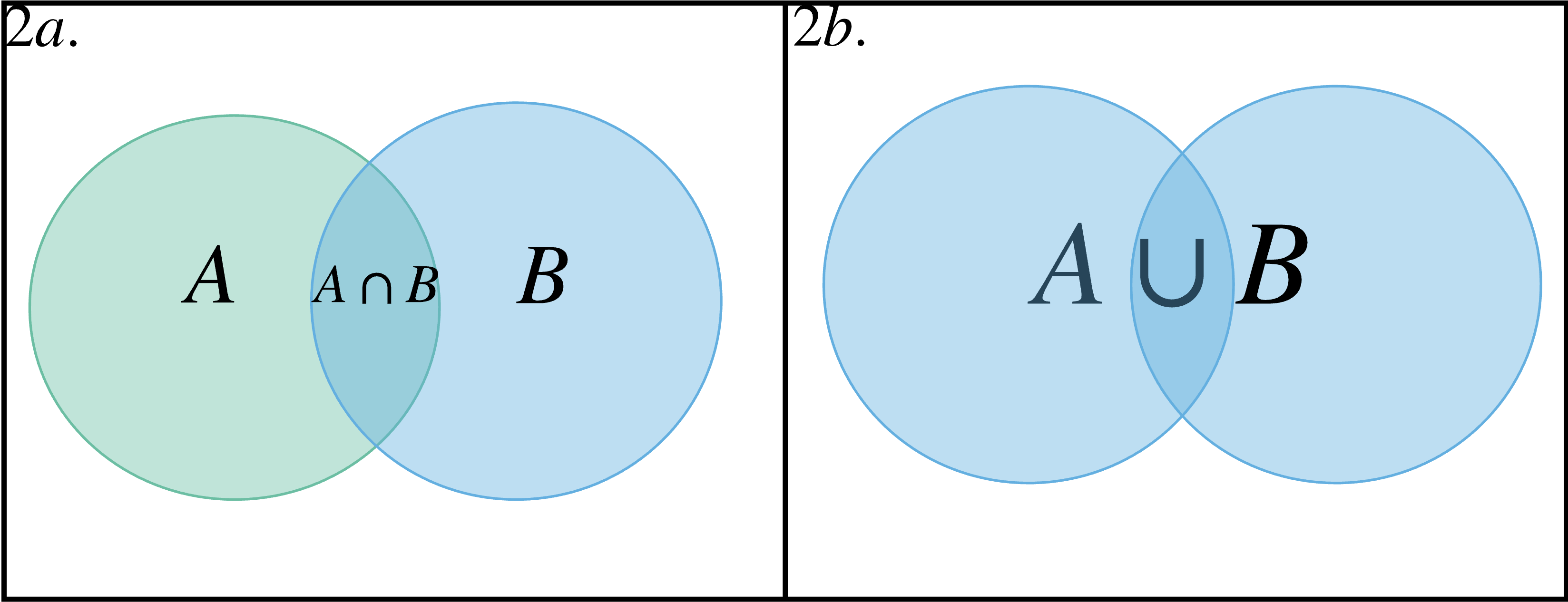
Now, let’s visualize the event space A as a circle, as in Figure 2. Any element in this circle is part of the set A that has a probability $P(A)$. Furthermore, let’s say we have a second event space where $B \in \mathcal{F_B}$ with elements in B also having probabilities $P(B)$. If we assume these circles intersected as in Figure 2, then the set intersection between the sets $A$ and $B$ is $A \cap B$. ⊕
Figure 2: The intersection of two sets can be visualized as the space at which they over overlap, shown in 2a. The union takes in account the rest of the elements in the other circles in addition to the intersection region.

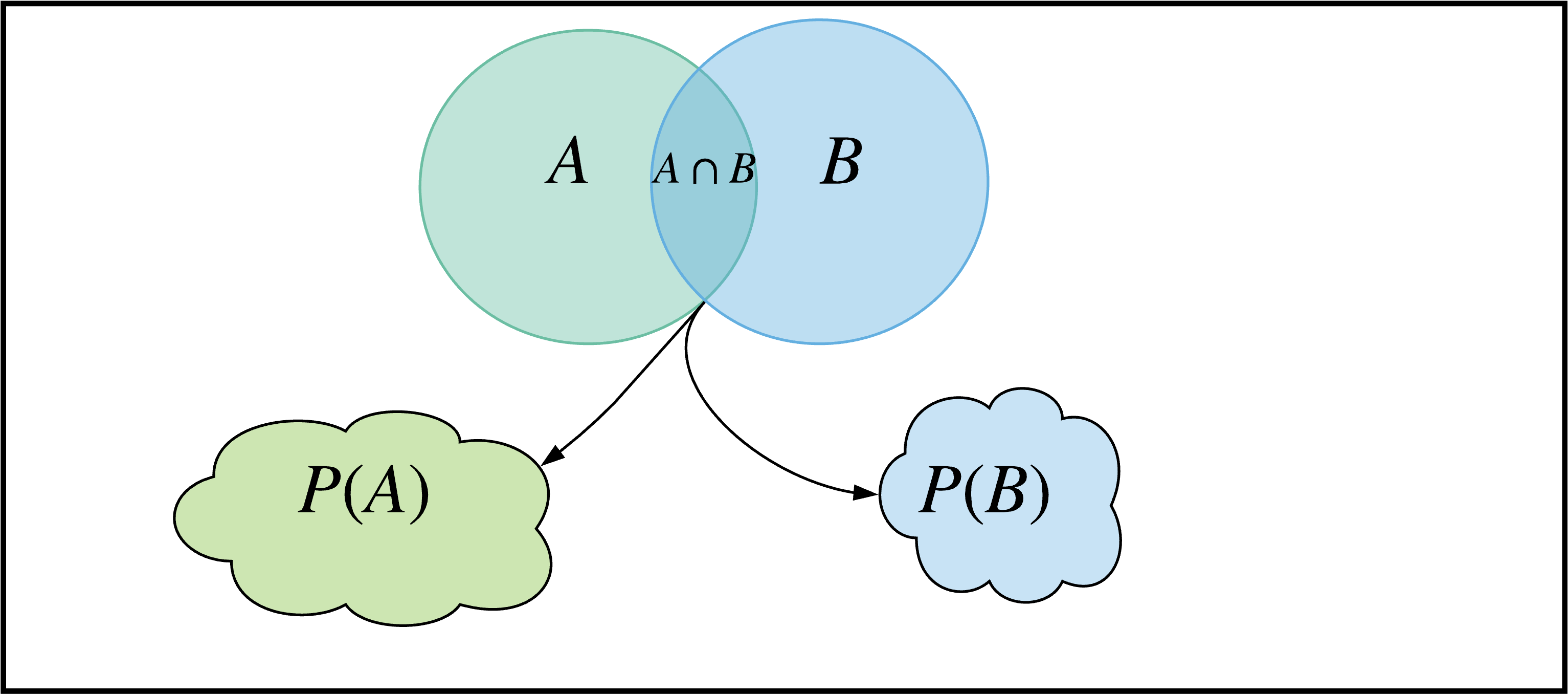
How do unions and intersections related to probabilities though? For instance, what is the proabability of the intersection? The probability of this intersection then just seems to be $P(A \cap B)$. But notice how this is ambiguous - the elements in this intersection can have probabilities mapped with respect to $P(A)$ and $P(B)$, as shown in Figure 3. So what are we trying to find with $P(A \cap B)$ - the probability of the intersection $A \cap B$ with respect to the probability mass function of $P(A)$ or $P(B)$? Both. We want to know the probability of getting this intersection with respect to $P(A)$ and $P(B)$. The probability of getting both requires us to first ask: does it matter if we get $P(A)$ before $P(B)$, or vice versa? If the answer is no, we say these two probability spaces are independent. ⊕
Figure 3: The intersected region between A and B map to two different probability spaces, P(A) and $P(B)$.

If they are independent, we then find the probability of getting P(A) by multiplying the elements in that intersection with respect to A, to the probabilities of those same elements in that intersection with respect to B $P(A \cap B) = P(A)P(B)$. But why do we multiply?

Imagine that the intersection between A and B, $A \cap B$, contains only one element. Furthermore, let’s say the probability of each element in A and B are $P(A)=\frac{1}{N}$ and $P(B)=\frac{1}{M}$, where N and M are the number of elements in A and B, respectively. The total number of possible combinations between all elements in A and B is the number of pairs we can make from them. Since each element of A can be paired to the entire space in B(ie. any element in A can be paired with all of B), the total number of pairs is $N \cdot M$. Getting this single pair that satisfies being the intersection between $A$ and $B$, $A \cap B$, is then $P(A \cap B) = \frac{1}{N \cdot M}$, which is the same as expressing this as $P(A \cap B) = \frac{1}{N \cdot M} = \frac{1}{N} \cdot \frac{1}{M} = P(A)P(B)$.

Similarly, let’s generalize this to have $A \cap B$ contain n elements in A and m elements in B. Now $P(A)=\frac{n}{N}$ and $P(B)=\frac{m}{M}$. Similarly, the total number of pairs is $N \cdot M$, while the number of pairs that intersect as $n \cdot m$, since for each element of a we can pair to an element in b. Finally, we get the same relationship that $P(A \cap B) = \frac{n \cdot m}{N \cdot M} = \frac{n}{N} \cdot \frac{m}{M} = P(A)P(B)$.

A different perspective to take is that we are creating an event space $\mathcal{F}$ that is composed of pairs between elements $A$ and $B$. That event space has a probability space $P(A \cup B)$ and $P(A \cap B)$ is just a subset as follows: $P((A \cap B) \in (A \cup B))$.

Example 1:
Let’s say the event space for A had two elements: one with even elements and the other with odd. The second event space B also had two elements, but these would one would have sample elements greater than 3 and the other would have equal to or less than 3. If we wanted the probaility of getting an even number that is ALSO greater than 3, then we have $P(A=\text{even} \cap B=\text{greater than 3})$. In the set intersection $(A=\text{even} \cap B=\text{greater than 3})$, we have $\{2,4,6\}$ and $\{4,5,6\}$ which satisfy the condition. Let these probabilities be $P(A=\{2,4,6\})=0.5$ and $P(B=\{4,5,6\})=0.5$. The probability of getting both requires us to ask: does it matter if we get $P(A=\{2,4,6\})$ before $P(B=\{4,5,6\})=0.5$, or vice versa? If the answer is no, we say these two are

Conditional Probabilities

Let’s try to understand what happens where event spaces are NOT independent; this is named Conditional Probability.

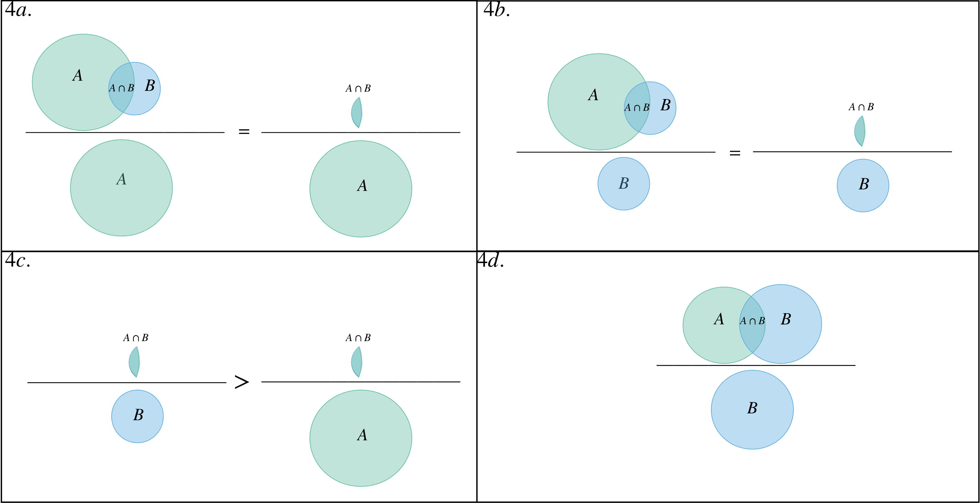
A central idea in probability is that probabilities are ratios between event spaces. If we go along this line of thinking, what happens if we take the ratio of getting the probability of the intersection between elements in A and B per probability of the elements in B in $P(A \cap B)$, hence $\frac{P(A \cap B)}{P(B)}$? We can see a visually clearer description in Figure 2. Given that A is much larger than B, $P(A \cap B)$ will account for a larger portion of $P(B)$ than it will for $P(A)$, hence $\frac{P(A \cap B)}{P(B)} > \frac{P(A \cap B)}{P(A)}$. ⊕
Figure 4: 4a and 4b show the visual representation of $\frac{P(A \cap B)}{P(A)}$ and $\frac{P(A \cap B)}{P(B)}$, respectively. 4c shows us that $\frac{P(A \cap B)}{P(B)} > \frac{P(A \cap B)}{P(B)}$. Lastly, we see that this representation is more difficult to see when the sizes of A and B are the same.

Mathematically, we have, $\frac{P(A \cap B)}{P(B)} = \frac{P(A') \cdot P(B')}{P(B)}$ for $A',B' \in A \cap B$. This just means the elements in A and B found in $A \cap B$ with their respective probability mappings, $P(A')$ and $P(B')$, relative to the all probabilitues in $P(B)$, defines what it means to be conditional. We write that the conditional probability of A with respect to B is:

\begin{equation} P(A \vert B) = \frac{P(A \cap B)}{P(B)} \end{equation}

Lastly, we can end with generalizing this conditional probability to an arbitrary number of event spaces as follows: