Introduction

Bayesian statistics is often daunting at first glance, however, its concepts are highly intuitive under graphical or geometric perspectives. To avoid any confusion from previous preconceptions, let’s begin with a complete a clean slate. This tabula rasa approach allows us to use mathematical descriptions as a way of enhancing our understanding, rather than trying to reverse engineer the logic behind these expressions.

Let’s begin with simple geometric area, and how we can begin our understanding of probabilities from their point of view. If we had two circles as in Figure 1A, area is just the measure of the enclosed space within these circular boundaries. If we had a machine that was able to shoot tiny particles completely random, then the probability of a particle ending up in the space of A is just the ratio of the area of A to the total area that makes up where ANY particle can end up in. If this were another circle, it would be the ratio of these two circular areas; The area of interest, A, is just a subset of this larger possible space.

⊕
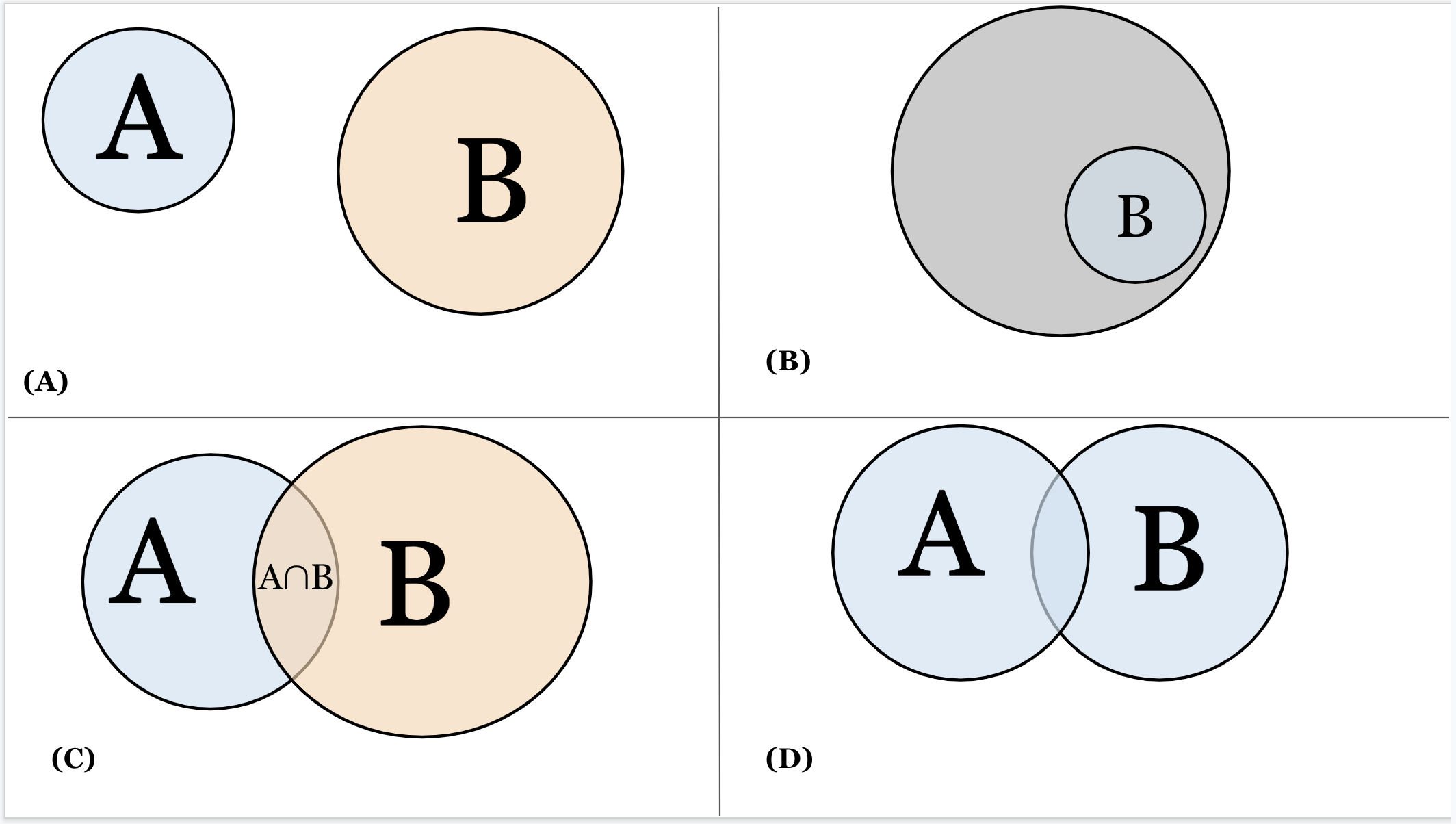
(A) Two distinct areas without intersections or unions. (B) If the gray circle is the complete area where a particle can end up in, the probability of a particle being in a subset area B is the ratio of that subset to the complete area. (C) An intersection is the shared area between A and B. The notation for intersection is often A∩B, A and B, A & B. (D) A union is the complete area of A and B together. The notation for intersection is often A∪B, A or B, A | B (not to be confused with a conditional in this last one).

</span>

Furthermore, let’s look at what happens when overlap these circles.

We don’t, or can’t, get the probability of a random variable, so we approximate. Frequentist statistics says we can express the probability of this random variable by taking the counts of the number of particles that hit inside the area,$n_x$, vs the total number, $n_t$. As the number of trials, $n_t$ goes to infinity, we should approach the ‘true’ probability.

$P(x) = \lim_{x \to \infty} \frac{n_x}{n_t}$.

If we think of having one particle and shooting it $n \to \infty$ times, then every trial is called an event. Furthermore, every event has an associated probability, where later events have better estimates of the true probability since they take into account the information of all previous events; probability converges over a large number of events.